Binary and Multi-class Semantic Classification Using EEGNet

This post will summarize my findings while testing EEGNet’s performance on binary and multiclass semantic classification of EEG data on a single subject of the THINGS-EEG dataset preprocessed by Dr. Gifford.

I implemented the EEGNet as described on the original paper (Lawhern et al.), using the recommended parameters of \(F_1=4\), \(D=2\) and dropout of \(0.5\). I also added a pipeline for training and printing the results to make the notebooks cleaner.

All code can be found at my GitHub (rfflrt) and was ran on a Nvidia RTX A5000.

Binary Classification on Single-Subject Data

In a binary dataset, the classes chosen to be discriminated alter greatly the accuracy achieved by EEGNet. As an example, given the classes “aircraft carrier” and “antelope” on sub-02:

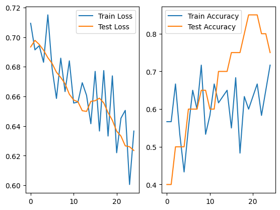
Achieving a accuracy of 0.85 on the best case.

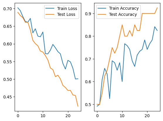
For the classes “balance beam” and “basson”, the accuracy was of 0.925 on the best case.

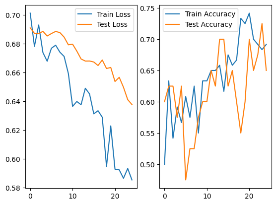
Although, for “aircraft carrier” and “ferry”, the best case was 0.725.

That way we may infer that semantically similar objects are more difficult to discriminate. Also, there may be ill-conditioning class separation, given that both aircraft carriers and ferries are waterborne vehicles.

The same observation can be made on the classes “fruit” against “orange” (where the best case was of 0.575 accuracy) and other similar cases.

Nina and I initially discussed congregating similar semantic classes as a single class, but I don’t think we will pursue this at the moment, since it would demand creating a robust criterion on what to merge and I also seek fine-grained discrimination that encompasses such nuances.

No significant variation was found when changing the subject I tested the EEGNet on.

Therefore, from this initial exploration, we could access:

• The EEGNet can, somewhat, discriminate between different semantic classes;
• If two classes are semantically similar (sometimes also geometrically or chromatically similar), the discrimination becomes harder;
• There are some ill-conditioned class separation on the dataset that may harm the results.

Multi-class Classification on Single-Subject Data

In a second exploration, given that there was no significant difference between the subjects considered, I explored multi-class (where I named “k-class” on the code) discrimination on the same dataset.

Clarifications

There are some details I may address in order to fully explain the performance findings.

The THINGS-EEG preprocessed by Dr. Gifford was not created in order to make semantic classification. In fact, it was done in order to align the encoding of images (the THINGS dataset) and EEG data, just like OpenAI’s CLIP, where the images were presented on a RSVP paradigm (which I will discuss after). This way, there are two sub-datasets inside the THINGS-EEG: the test and the training datasets. In general, there are 10 subjects and each image has a (17,100) matrix representing the channels $\times$ time stimulus. The training dataset is composed by:

• 1654 classes
• 10 images per class
• 4 repetitions of each image that way, each class has 40 stimuli per subject for the model to train on, what is very scarse data. The test dataset is composed by:
• 200 classes
• 1 image per class
• 80 repetitions of each image that way, each class has 80 stimuli per subject, which is the double of the training dataset but is still a low number.

It is important to note that the classes of the training and test datasets are disjoint, what means there is no way for us to congregate the data in a meaningful way without unbalancing classes or curating it as Nina and I discussed before.

For more precision and to avoid mixing the THINGS-EEG training and testing subdatasets with the data used to train and test the model, let us assume:

• Dataset A as the THINGS-EEG training subdataset
• Dataset B as the THINGS-EEG testing subdataset

Results

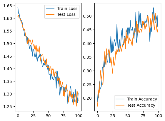
Using the data of sub-01 in a 3/4 separation of the data for train and 1/4 for test, the performance of the EEGNet on the first 5 classes of the A dataset was:

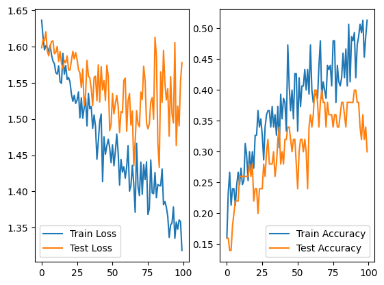
We can see that the loss on the training and testing data was highly unstable and, considering their distance increasing also observed on the accuracy, we may infer that the model was already overfitting without even achieving good metrics. The accuracy on the best case was 0.4 and was constantly above 0.2, which indicates that it is better than a simple uniform distribution, but is still poor and unreliable.

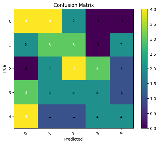
The confusion matrix makes it clear that the performance is not as good as we would like, since the main diagonal, though somewhat clear, not enough from the rest of the matrix.

Using the B dataset with the same separation, we got the results:

Now, we see that the loss in both the train and test data is more stable and descend without great differences in distance, starting to achieve a plateau. The same characteristics can be seen on the accuracy curve. Obtaining an accuracy of 0.55 on the best case, we observe an increase on the performance and reliability when using more data.

It is good to also observe that the variability of the dataset also decreases, since the A dataset uses 10 different stimuli, while the B uses only 1. This may indicate that the increasing of quantitative and qualitative observations were due to this reducing of variance, what we will show in the future is not the case.

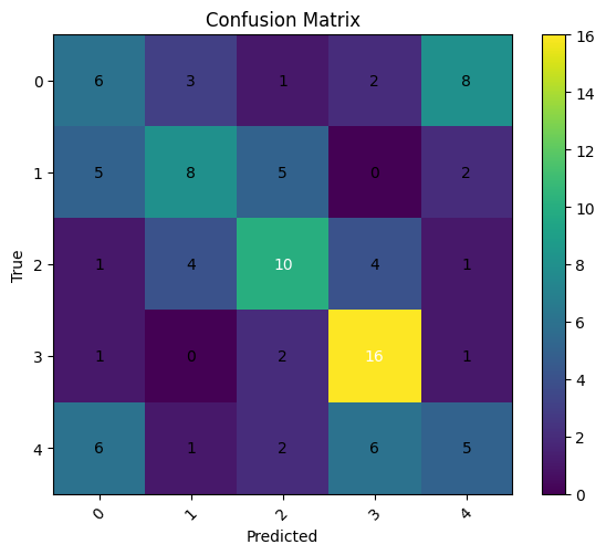
We observe a better formation of the main diagonal, though still not very good, with a good discrimination of the “balance beam” class and poor discrimination of the “banana” and “aircraft carrier” classes, which the model, strangely, confuses itself with.